Get Certified for
Commercial Banking (CBCA®)
Stand out and gain a competitive edge as a commercial banker, loan officer, or credit analyst with advanced knowledge, real-world analysis skills, and career confidence.
This Microsoft Excel template illustrates how to create a loan amortization schedule, as well as dealing with additional payments and variable interest rates
Whether buying a car or house or paying down a credit card, knowing how to calculate a loan payment is key when considering your financial options.
An amortization schedule is often provided to illustrate when a loan is paid off, as well as to show the remaining loan balance after every payment. This schedule shows loan and payment details for an amortizing term loan. An amortizing loan is repaid via periodic installments over the lifetime of the loan. Installments are typically equal monthly payments, but not always. Each periodic payment includes both a principal portion and an interest portion.
In this article, we will show how to calculate a payment and create a loan amortization schedule in Excel.
Download the free Amortization Schedule Template now to advance your knowledge.
For the purposes of this template, we will assume that payments are made monthly, and we will begin by assuming that each payment is for the same amount. Equal monthly payments would be the case if the interest rate is fixed and there are no additional principal reductions.
As mentioned earlier, each payment consists of an interest portion and a principal portion. The interest portion of an amortizing term loan is higher at the beginning of the loan than at the end. This is because the loan’s principal is reduced over the life of the loan, resulting in lower interest expense as the loan reaches maturity.
The formula for calculating the payment of an amortizing loan is:
Fortunately, we don’t have to memorize that formula since Excel has the handy PMT function we can use instead.
The PMT function uses the following syntax: PMT(rate, nper, pv, [fv], [type]). The first three arguments are required and what we will focus on.
With a monthly payment schedule, we will need to make sure we convert any annual numbers to monthly. Since interest rates are quoted in annual terms, we will need to convert this rate to a monthly rate by dividing by 12. Likewise, if a loan is quoted in years, we will need to multiply the number of years by 12 to calculate the monthly payment properly.
The PMT function will automatically output the result as a negative number unless we make the loan amount negative or enter the entire function with a “minus” sign in front of it.
For example, assume the loan amount is $100,000, with an annual interest rate of 7 percent and a one-year (12-month) term. We would enter that into the PMT function as =PMT(.07/12,12,-100000), resulting in $8,652.67.
However, as part of a loan amortization schedule, we need to separate the monthly payments into the interest part and principal part.
The interest part of the loan payment is calculated using the beginning balance of the loan. In other words, the formula is:
The beginning loan amount changes each month since a portion of the principal balance is being repaid as part of the monthly payment.
Alternatively, we can use Excel’s IPMT function, which has the following syntax: =IPMT(rate, per, nper, pv, [fv], [type]). Again, we are focused on the required arguments:
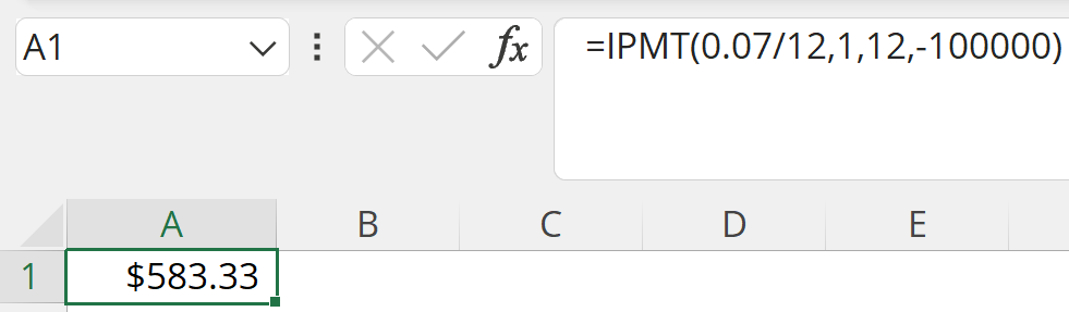
Continuing our earlier example, assume the loan amount is $100,000, with an annual interest rate of 7 percent. Further, assume we want the interest amount in the first month and the loan matures in 12 months. We would enter that into the IPMT function as =IPMT(.07/12,1,12,-100000), resulting in $583.33.
If we were instead looking for the interest portion in the second month, we would enter =IPMT(.07/12,2,12,-100000), resulting in $536.26.
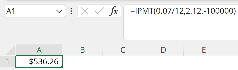
The interest portion of the payment is lower in the second month since a portion of the loan amount was paid down in the first month.
After calculating the full monthly payment and the amount of interest, the difference between the two numbers is the principal paydown amount.
Using our earlier example, the principal paydown in the first month is the difference in the total payment amount of $8,652.67 and the interest payment of $583.33, or $8,069.34.
Alternatively, we can also use the PPMT function to calculate this amount. The PPMT syntax is =PPMT( rate, per, nper, pv, [fv], [type]). We will focus on the four required arguments:
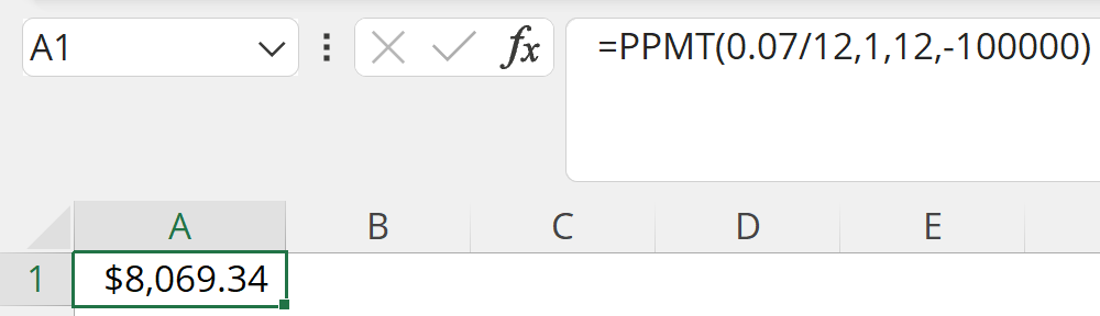
Again, assume the loan amount is $100,000, with an annual interest rate of 7 percent. Further, assume we want the principal amount in the first month and the loan matures in 12 months. We would enter that into the PPMT function as =PPMT(.07/12,1,12,-100000), resulting in $8,069.34.
If we were instead looking for the principal portion in the second month, we would enter =PPMT(.07/12,2,12,-100000), resulting in $8,116.41.
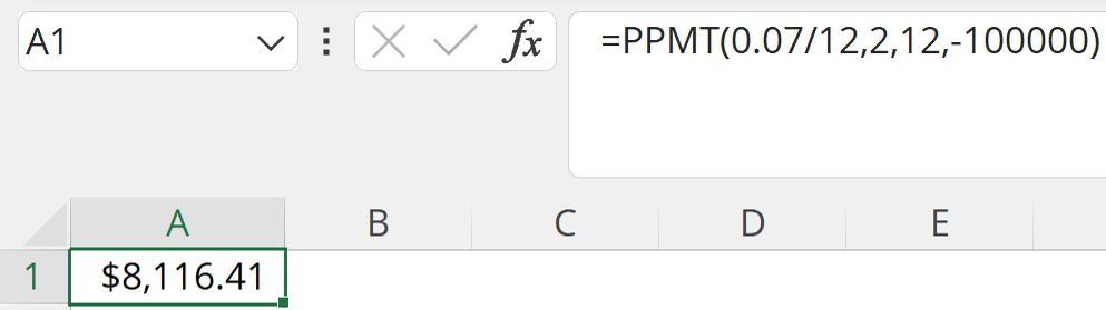
Since we just calculated the second month’s interest part and principal part, we can add the two and see the total monthly payment is $8,652.67 ($536.26 + $8,116.41), which is exactly what we calculated earlier.
Instead of hardcoding those numbers into individual cells in a worksheet, we can put all of that data into a dynamic Excel spreadsheet and use that to create our amortization schedule.
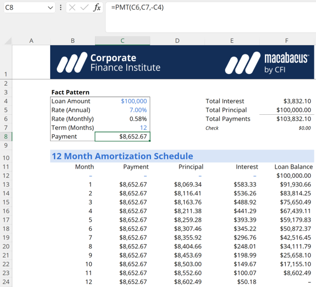
The above screenshot shows a simple 12-month loan amortization schedule in our downloadable template. This amortization schedule is on the worksheet labeled Fixed Schedule. Note that each monthly payment is the same, the interest part decreases over time as more of the principal part is paid, and the loan is fully repaid by the end.
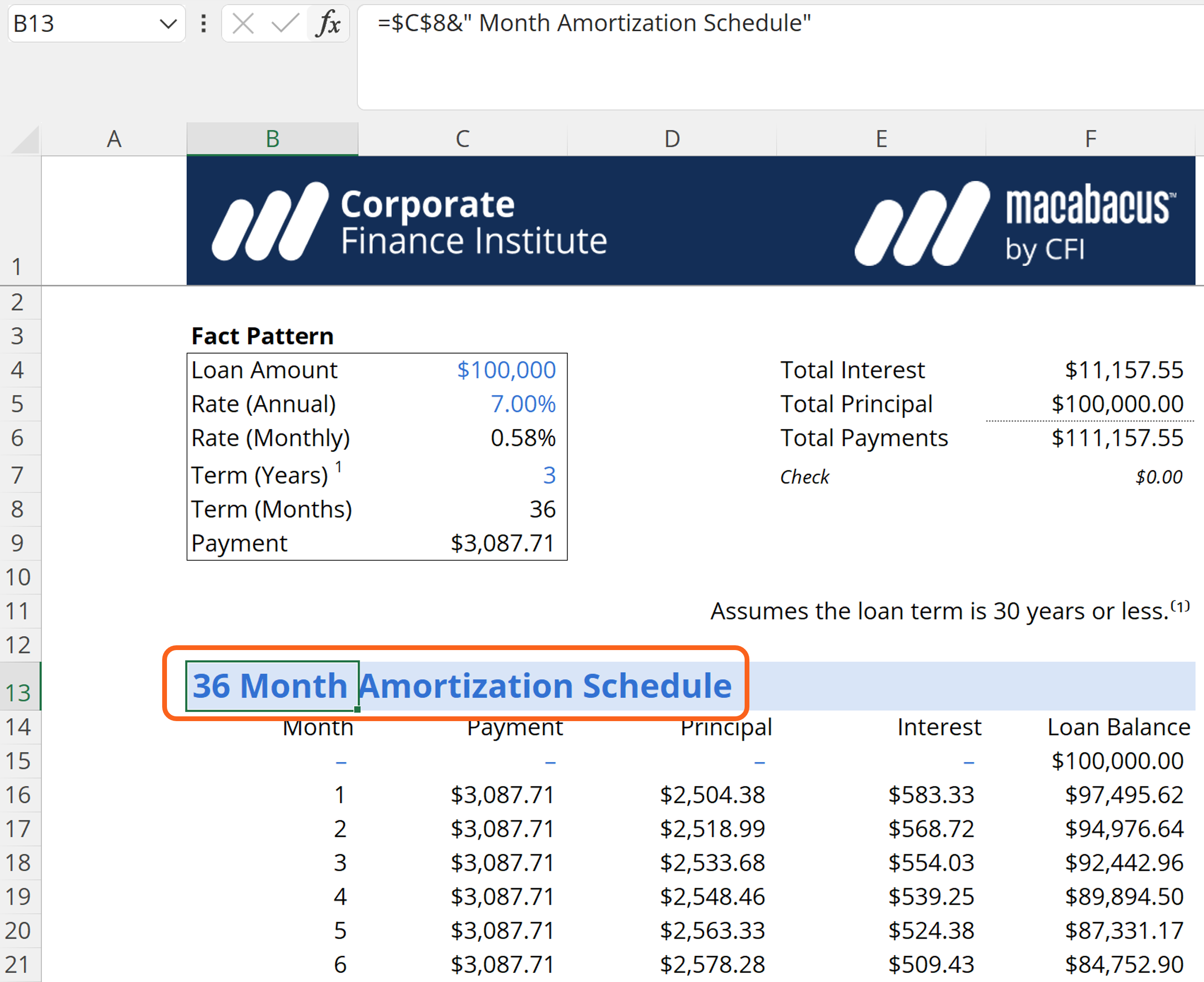
Of course, many amortizing term loans are longer than one year, so we can further enhance our worksheet by adding more periods and hiding those periods that are not in use.
To make this more dynamic, we will create a dynamic header using the ampersand (“&”) symbol in Excel. The ampersand symbol is equivalent to using the CONCAT function. We can then change the loan term and the header will update automatically, as shown below.

Additionally, if we want to create a variable-period loan amortization schedule, we probably don’t want to show all of the calculations for periods outside of our amortization. For example, if we set up our schedule for a maximum 30-year amortization period, but we only want to calculate a two-year period, we can use Excel’s Conditional Formatting to hide the 28 years we don’t need.
First, we will select the entire maximum range of our amortization calculator. In the Excel template, the maximum amortization range on the Variable Periods worksheet is B15 to F375 (30 years of monthly payments).
From there, go to Home on the Excel ribbon, select Conditional Formatting, then New Rule. We’ll then use a formula to determine which cells to format. In this case, we base everything on the number of months we DO want to see in our schedule. For months we DON’T want to see we can change the font color to white so that it’s not visible (assuming the worksheet uses the default white background).
For the Conditional Formatting rule, we will test to see if the value in column B is greater than or equal to the total number of months we want to see. We add 1 at the end of the formula (see the screenshot below) to account for month “zero,” where there is no payment.

We also want to make sure the anchoring is set up properly: we want to fully anchor cell C8 since we will always want to reference that cell (the total number of months). However, we only want to anchor column B since that column contains the month number used to calculate the interest and principal payments.

Basically, the Conditional Formatting new rule is saying if whatever in column B is greater than or equal to the total number of months in cell C8 (plus 1 to account for month “zero”), then we want to change the font color to white so that it effectively “hides” the values and calculations in those cells.
For additional assurance, we also modify all calculations to return a blank cell if the specific month number is greater than the number in cell C8. For example, the first month’s interest payment in cell E16 has been modified to =IF(B16<=$C$8,IPMT($C$6,B16,$C$8,-$C$4),””). This relatively simple IF statement is tested to see if a specific month number is less than the total number of months. If this argument is True, the IPMT function returns the proper value. Otherwise, the IF statement returns a blank cell, which can be created in Excel by using double quotes (“”).
This Excel template also allows a user to enter extra payments that are used to pay down additional principal. Since the principal is being paid down even faster, then the loan will be repaid before its stated maturity. However, this does require substantial modifications from the previous worksheets.
On the worksheet titled Additional Principal Paydown, note that we’ve added an additional principal paydown of $500 per month. If a user wants to vary the extra payments, then those payments can just be entered directly into the appropriate month. Otherwise, our template assumes the $500 extra payment is made every month (or at least until the remaining principal balance is less than $500).
As you can see below, we use an IF statement to pull in the additional payment. The calculation ensures the additional payment is only made if the additional payment is less than the previous month’s loan balance (less the current month’s principal portion).

Additionally, because there is an additional payment, we no longer use the IPMT and PPMT functions. Instead, we calculate the interest portion using our earlier formula: Annual Interest Rate/12 * Beginning Loan Amount. The principal payment is the scheduled payment less the interest.
The loan balance has also been modified. Like the previous worksheets, the loan balance is reduced by the principal part of the scheduled payment, but we also need to reduce the loan balance by the additional principal paydown.

Finally, our template can also take into account changing interest rates. In this case, we have set up the loan amortization schedule so that a user can enter the new interest rate (in annual terms) in the months in which the interest rate applies. The variable rate schedule is on the worksheet titled Variable Interest Rate.
In this case, all of the calculations from the Additional Principal Paydown worksheet apply, but we’ve modified the scheduled payment calculation.
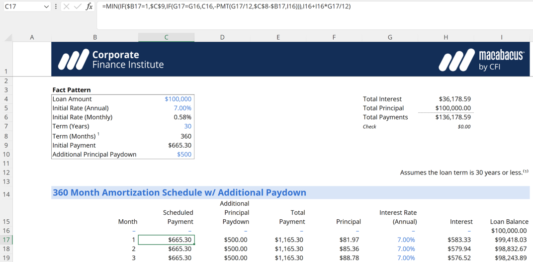
The formula in the above screenshot is basically saying if we’re in the first month, then reference the initial payment. Otherwise, we check to see if the interest rate has changed. If it has not changed, then we reference the cell right above to maintain the same scheduled payment.
However, if the interest rate changes, we use the PMT function to obtain the new scheduled payment. We finish the formula by wrapping it in a MIN function. This will ensure our payment will go to zero once the loan has been repaid.


