Adjusted R-squared

What is the Adjusted R-squared?

The adjusted R-squared is a modified version of R-squared that accounts for predictors that are not significant in a regression model. In other words, the adjusted R-squared shows whether adding additional predictors improve a regression model or not. To understand adjusted R-squared, an understanding of R-squared is required.

What is the R-squared?

The R-squared, also called the coefficient of determination, is used to explain the degree to which input variables (predictor variables) explain the variation of output variables (predicted variables). It ranges from 0 to 1. For example, if the R-squared is 0.9, it indicates that 90% of the variation in the output variables are explained by the input variables. Generally speaking, a higher R-squared indicates a better fit for the model. Consider the following diagram:

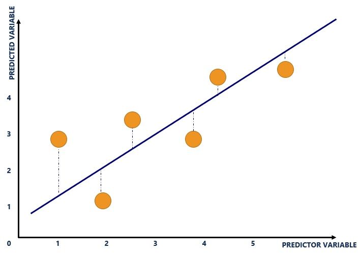
The blue line refers to the line of best fit and shows the relationship between variables. The line is calculated through regression analysis and is plotted where the vertical distances (blue dotted lines) of the yellow dots to the line of best fit is minimized.

The yellow dots refer to the plot of input and output variables. The input variable is plotted on the x-axis while the output variable is plotted on the y-axis. For example, the graph above consists of the following dataset:

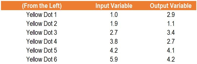
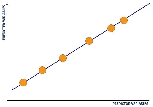
The blue dotted lines refer to the distance of the plot of input and output variables from the line of best fit. The R-squared is derived from the distance of all the yellow dots from the line of best fit (the blue line). For example, the following diagram would illustrate an R-squared of 1:

Problems with the R-squared

R-squared comes with an inherent problem – additional input variables will make the R-squared stay the same or increase (this is due to how the R-squared is calculated mathematically). Therefore, even if the additional input variables show no relationship with the output variables, the R-squared will increase. An example that explains such an occurrence is provided below.

Understanding the Adjusted R-squared

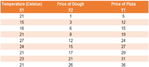
Essentially, the adjusted R-squared looks at whether additional input variables are contributing to the model. Consider an example using data collected by a pizza owner, as shown below:

Assume the pizza owner runs two regressions:

Regression 1: Price of Dough (input variable), Price of Pizza (output variable)

Regression 1 yields an R-squared of 0.9557 and an adjusted R-squared of 0.9493.

Regression 2: Temperature (input variable 1), Price of Dough (input variable 2), Price of Pizza (output variable)

Regression 2 yields an R-squared of 0.9573 and an adjusted R-squared of 0.9431.

Although temperature should not exert any predictive power on the price of a pizza, the R-squared increased from 0.9557 (Regression 1) to 0.9573 (Regression 2). A person may believe that Regression 2 carries higher predictive power since the R-squared is higher. Even though the input variable of temperature is useless in predicting the price of a pizza, it increased the R-squared. Here, the adjusted R-squared comes in.

The adjusted R-squared looks at whether additional input variables are contributing to the model. The adjusted R-squared in Regression 1 was 0.9493 compared to the adjusted R-squared in Regression 2 of 0.9493. Therefore, the adjusted R-squared is able to identify that the input variable of temperature is not helpful in explaining the output variable (the price of a pizza). In such a case, the adjusted R-squared would point the model creator to using Regression 1 rather than Regression 2.

Example of the Adjusted R-squared

Consider two models:

• Model 1 uses input variables X1, X2, and X3 to predict Y1.
• Model 2 uses input variables X1 and X2 to predict Y1.

Which model should be used? Information regarding both models is provided below:

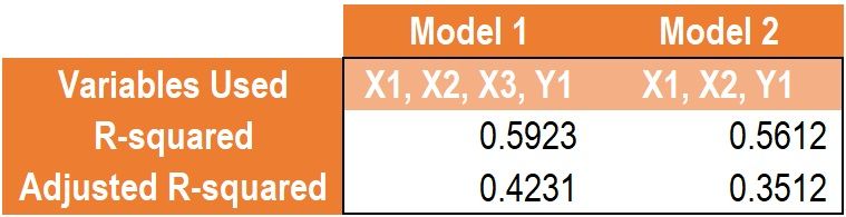
Comparing the R-squared between Model 1 and Model 2, the R-squared predicts that Model 1 is a better model as it carries greater explanatory power (0.5923 in Model 1 vs. 0.5612 in Model 2).

Comparing the R-squared between Model 1 and Model 2, the adjusted R-squared predicts that the input variable X3 contributes to explaining output variable Y1 (0.4231 in Model 1 vs. 0.3512 in Model 2).

As such, Model 1 should be used, as the additional X3 input variable contributes to explaining the output variable Y1.

Additional Resources

Thank you for reading CFI’s guide to Adjusted R-squared. To keep learning and advancing your career, the following CFI resources will be helpful:

• Free Data Science Course
• Basic Statistics Concepts for Finance
• High-Low Method vs. Regression Analysis
• Independent Variable
• Types of Financial Analysis
• See all data science resources