Get Certified for
Capital Markets (CMSA®)
From equities and fixed income to derivatives, the CMSA certification bridges the gap from where you are now to where you want to be — a world-class capital markets analyst.
Calculate the theoretical value of an option
Option Pricing Models are mathematical models that use certain variables to calculate the theoretical value of an option. The theoretical value of an option is an estimate of what an option should be worth using all known inputs. In other words, option pricing models provide us a fair value of an option.
Knowing the estimate of the fair value of an option, finance professionals could adjust their trading strategies and portfolios. Therefore, option pricing models are powerful tools for finance professionals involved in options trading.
A formal definition of an option states that it is a type of contract between two parties that provides one party the right, but not the obligation, to buy or sell the underlying asset at a predetermined price before or at expiration day. There are two major types of options: calls and puts.
Options may also be classified according to their exercise time:
The above-mentioned classification of options is extremely important because choosing between European-style or American-style options will affect our choice for the option pricing model.
Before we start discussing different option pricing models, we should understand the concept of risk-neutral probabilities, which are widely used in option pricing and may be encountered in different option pricing models.
The risk-neutral probability is a theoretical probability of future outcomes adjusted for risk. There are two main assumptions behind this concept:
The risk-neutral probability is the probability that the stock price would rise in a risk-neutral world. However, we neither assume that all the investors in the market are risk-neutral, nor the fact that risky assets will earn the risk-free rate of return. This theoretical value measures the probability of buying and selling the assets as if there was a single probability for everything in the market.
The simplest method to price the options is to use a binomial option pricing model. This model uses the assumption of perfectly efficient markets. Under this assumption, the model can price the option at each point of a specified time frame.
Under the binomial model, we consider that the price of the underlying asset will either go up or down in the period. Given the possible prices of the underlying asset and the strike price of an option, we can calculate the payoff of the option under these scenarios, then discount these payoffs and find the value of that option as of today.
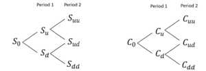
Figure 1. Two-period binomial tree
The Black-Scholes model is another commonly used option pricing model. This model was discovered in 1973 by the economists Fischer Black and Myron Scholes. Both Black and Scholes received the Nobel Memorial Prize in economics for their discovery.
The Black-Scholes model was developed mainly for pricing European options on stocks. The model operates under certain assumptions regarding the distribution of the stock price and the economic environment. The assumptions about the stock price distribution include:
The assumptions about the economic environment are:
Nevertheless, these assumptions can be relaxed and adjusted for special circumstances if necessary. In addition, we could easily use this model to price options on assets other than stocks (currencies, futures).
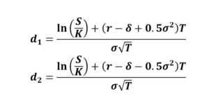
The main variables used in the Black-Scholes model include:

From the Black-Scholes model, we can derive the following mathematical formulas to calculate the fair value of the European calls and puts:
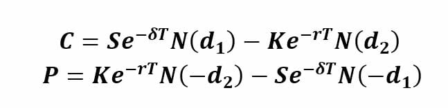
The formulas above use the risk-adjusted probabilities. N(d1) is the risk-adjusted probability of receiving the stock at the expiration of the option contingent upon the option finishing in the money. N(d2) is the risk-adjusted probability that the option will be exercised. These probabilities are calculated using the normal cumulative distribution of factors d1 and d2.
The Black-Scholes model is mainly used to calculate the theoretical value of European-style options and it cannot be applied to the American-style options due to their feature to be exercised before the maturity date.
Monte-Carlo simulation is another option pricing model we will consider. The Monte-Carlo simulation is a more sophisticated method to value options. In this method, we simulate the possible future stock prices and then use them to find the discounted expected option payoffs.
In this article, we will discuss two scenarios: simulation in the binomial model with many periods and simulation in continuous time.
Under the binomial model, we consider the variants when the asset (stock) price either goes up or down. In the simulation, our first step is determining the growth shocks of the stock price. This can be done through the following formulas:
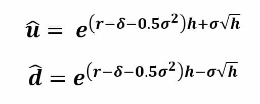
h in these formulas is the length of a period and h = T/N and N is a number of periods.
After finding future asset prices for all required periods, we will find the payoff of the option and discount this payoff to the present value. We need to repeat the previous steps several times to get more precise results and then average all present values found to find the fair value of the option.
In the continuous time, there is an infinite number of time points between two points in time. Therefore, each variable carries a particular value at each point in time.
Under this scenario, we will use the Geometric Brownian Motion of the stock price which implies that the stock follows a random walk. Random walk means that the future stock prices cannot be predicted by the historical trends because the price changes are independent of each other.
In the Geometric Brownian Motion model, we can specify the formula for stock price change:
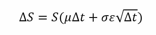
Where:
S – stock price
ΔS – change in stock price
µ – expected return
t – time
σ – standard deviation of stock returns
↋ – random variable µ
Unlike the simulation in a binomial model, in continuous time simulation, we do not need to simulate the stock price in each period, but we need to determine the stock price at the maturity, S(T), using the following formula:
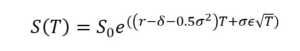
We generate the random number ↋ and solve for S(T). Afterward, the process is similar to what we did for simulation in the binomial model: find the option’s payoff at the maturity and discount it to the present value.
Connect what you just learned to a clear career path with CFI’s role‑based courses and certification programs.
Thank you for reading CFI’s guide on Option Pricing Models. To keep advancing your career, the additional CFI resources below will be useful:


