Get Certified for
Business Intelligence (BIDA®)
Develop analytical superpowers by learning how to use programming and data analytics tools such as VBA, Python, Tableau, Power BI, Power Query, and more.
Also known as Gaussian or Gauss distribution
The normal distribution is also referred to as the Gaussian or Gauss distribution. The distribution is widely used in natural and social sciences. It is made relevant by the Central Limit Theorem, which states that the averages obtained from independent, identically distributed random variables tend to form normal distributions, regardless of the type of distributions they are sampled from.
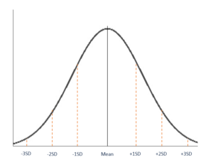
A normal distribution is symmetric from the peak of the curve, where the mean is. This means that most of the observed data is clustered near the mean, while the data become less frequent when farther away from the mean. The resultant graph appears as bell-shaped where the mean, median, and mode are of the same values and appear at the peak of the curve.
The graph is a perfect symmetry, such that, if you fold it at the middle, you will get two equal halves since one-half of the observable data points fall on each side of the graph.
The two main parameters of a (normal) distribution are the mean and standard deviation. The parameters determine the shape and probabilities of the distribution. The shape of the distribution changes as the parameter values change.
The mean is used by researchers as a measure of central tendency. It can be used to describe the distribution of variables measured as ratios or intervals. In a normal distribution graph, the mean defines the location of the peak, and most of the data points are clustered around the mean. Any changes made to the value of the mean move the curve either to the left or right along the X-axis.
The standard deviation measures the dispersion of the data points relative to the mean. It determines how far away from the mean the data points are positioned and represents the distance between the mean and the observations.
On the graph, the standard deviation determines the width of the curve, and it tightens or expands the width of the distribution along the x-axis. Typically, a small standard deviation relative to the mean produces a steep curve, while a large standard deviation relative to the mean produces a flatter curve.
All forms of (normal) distribution share the following characteristics:
A normal distribution comes with a perfectly symmetrical shape. This means that the distribution curve can be divided in the middle to produce two equal halves. The symmetric shape occurs when one-half of the observations fall on each side of the curve.
The middle point of a normal distribution is the point with the maximum frequency, which means that it possesses the most observations of the variable. The midpoint is also the point where these three measures fall. The measures are usually equal in a perfectly (normal) distribution.
In normally distributed data, there is a constant proportion of distance lying under the curve between the mean and specific number of standard deviations from the mean. For example, 68.25% of all cases fall within +/- one standard deviation from the mean. 95% of all cases fall within +/- two standard deviations from the mean, while 99% of all cases fall within +/- three standard deviations from the mean.
Skewness and kurtosis are coefficients that measure how different a distribution is from a normal distribution. Skewness measures the symmetry of a normal distribution while kurtosis measures the thickness of the tail ends relative to the tails of a normal distribution.
Most statisticians give credit to the French scientist Abraham de Moivre for the discovery of normal distributions. In the second edition of “The Doctrine of Chances,” Moivre noted that probabilities associated with discretely generated random variables could be approximated by measuring the area under the graph of an exponential function.
Moivre’s theory was expanded by another French scientist, Pierre-Simon Laplace, in “Analytic Theory of Probability.” Laplace’s work introduced the central limit theorem that proved that probabilities of independent random variables converge rapidly to the areas under an exponential function.
Connect what you just learned to a clear career path with CFI’s role‑based courses and certification programs.
Thank you for reading CFI’s guide on Normal Distribution. To keep learning and advancing your career, the additional CFI resources below will be useful:


