Lognormal Distribution

What is Lognormal Distribution?

A lognormal distribution is common in statistics and probability theory. Lognormal distribution is also known as the Galton or Galton’s distribution, being named after Francis Galton, a statistician during the English Victorian Era.

By definition, the lognormal distribution is the discrete and ongoing distribution of a random variable, the logarithm of which is normally distributed. In other terms, lognormal distribution follows the concept that instead of having the original raw data normally distributed, the logarithms of this raw data that are computed are also normally distributed.

Understanding Lognormal Distribution

A lognormal distribution is a result of the variable “x” being a product of several variables that are identically distributed. It is common in statistics that data be normally distributed for statistical testing. The lognormal distribution can be converted to a normal distribution through mathematical means and vice versa.

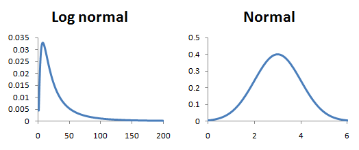
The image below shows the lognormal distribution and normal distribution:

The lognormal distribution consists of only positive values and follows the notation:

ln(x₁), ln(x₂), ln(x₃), etc.,

where the original variables are:

x₁, x₂, x₃, etc.

Some common applications of lognormal distributions include maintenance data analysis (for example, the time it may take to repair a specific piece of equipment) and economic and/or stock market data analysis (where positive values may be required to determine future returns for a stock).

The lognormal distribution is an ideal model for processes where the multiplication of effects results in time to failure. The model is considered to be very useful in the fields of medicine, economics, and engineering.

Normal Distribution

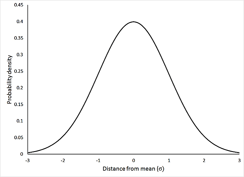
Normal distribution is a term that is popular in statistics and is used to describe how the values in a data set are distributed. A normal distribution is a symmetric distribution, as seen in the chart below:

Normal distribution is considered one of the most important probability distributions due to its versatility and ability to accommodate different phenomena or events – e.g., height, test results, measurement errors, etc. The two measures of normal distribution are the mean (which is used to determine central tendency) and the standard deviation (which is used to determine the distance between recorded values and the mean).

The common properties of normal distributions are:

• Normal distributions are symmetrical and not skewed.
• The descriptive measures are normal (mean, median, and mode).
• Half of the population is greater than the mean, and the other half is lesser than the mean.

Normal distribution is pivotal in statistics because hypothesis testing follows the assumption that data is normally distributed, and regression (linear and non-linear) follows the assumption that residuals are normally distributed. In conjunction with the Central Limit Theorem, it is argued that when a sample size increases, the distribution of the sample’s mean is normally distributed, despite the possibility of seeing the original values not being normally distributed.

Testing for Normality

Normality assumes that data (once plotted or charted) forms a symmetric bell curve. Normality is needed for regression and other statistical tests. One can test for normality by using a graph and analyzing its shape or through statistics tests such as the Shapiro-Wilk Test, Jarque-Bera Test, D’Agostino-Pearson Test, Kolmogorov-Smirnov Goodness of Fit Test, and among others, the Chi-square normality test.

Lognormal vs. Normal Distribution

Lognormal distributions tend to be used together with normal distributions, as lognormal distribution values are derived from normally distributed values through mathematical means. One key difference between the two is that lognormal distributions contain only positive numbers, whereas normal distribution can contain negative values.

Another key difference between the two is the shape of the graph. Normally distributed data forms a symmetric bell-shaped graph, as seen in the previous graphs. In contrast, lognormally distributed data does not form a symmetric shape but rather slants or skews more towards the right.

Additional Resources

Thank you for reading CFI’s guide to Lognormal Distribution. To keep learning and advancing your career, the following resources will be helpful:

• Basic Statistics Concept in Finance
• Distribution Yield
• Descriptive Statistics
• Hypothesis Testing
• LOGNORM.INV Function
• See all data science resources