Get Certified for Financial Modeling (FMVA)®
Gain in-demand industry knowledge and hands-on practice that will help you stand out from the competition and become a world-class financial analyst.
A modified form of Net Present Value (NPV) that takes into account the present value of leverage effects separately
APV (Adjusted Present Value) is a modified form of Net Present Value (NPV) that takes into account the present value of leverage effects separately. APV splits financing and non-financing cash flows and discounts them separately. It is a more flexible valuation tool to show benefits, such as tax shields, arising from tax deductions of interest and costs, such as financial distress. The formula for APV is as follows:
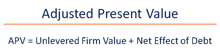
The net effect of debt includes adjustments such as the present value of interest tax shields, debt issuance costs, financial distress costs, and other financial side effects.
APV is an appropriate measure of value for many situations, including:
The APV approach is more superior in such situations since they involve complex debt assumptions.
The typical Net Present value (NPV) approach bakes all the debt assumptions into the cost of debt, which flows into the weighted average cost of capital (WACC). However, WACC is an inflexible discount rate that does not consider many financial side effects, such as financial distress, future interest tax shields, etc. Furthermore, WACC applies the discount rate to levered cash flows that are available for both equity and debt holders.
The Adjusted Present Value (APV) distinguishes the levered and unlevered cash flows and discounts them separately, giving a more accurate depiction of costs of equity and debt and cash flows available for both equity and debt holders.
Unlevered cash flows are discounted at the unlevered cost of capital, which can be calculated with the capital asset pricing model (CAPM).

Calculate the present value of debt financing assumptions.
As with any Discounted Cash Flow (DCF) valuation, start with the forecasted cash flows for a company, business line, or project. The cash flows should be the unlevered cash flows that are available to just equity holders. It considers after-tax operating cash flows, changes in net working capital, capital expenditures, and other changes in assets after-tax.
The forecasted cash flows cannot be forecasted too far out in time, or it will be inaccurate. Instead, a terminal value assumption is made for the perpetual cash flows after the forecasted period. It can be done with a few methods, including:
With the Gordon Growth Model, the perpetual cash flows are calculated with a perpetual formula that assumes a perpetual growth rate, and cost of capital that is applied to the last year’s forecasted cash flow.
With the multiples method, a multiple such as TV/EBITDA or TV/EBIT is applied to the last forecasted year. The multiple can be calculated by taking the average of comparable companies multiples in comparable company analysis.
The forecasted cash flows and terminal value should be discounted to the present value with an appropriate discount rate. The discount rate should accurately reflect the opportunity cost of capital for equity holders, i.e., the expected return on an asset with similar risk characteristics. The discounted cash flows represent the unlevered present value of the subject.
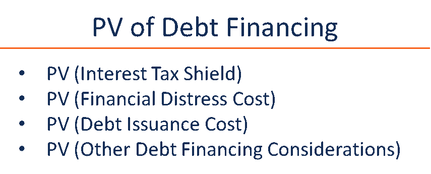
The present value of side effects arising from the use of leverage should be calculated. The most common side effect to evaluate is the interest tax shield. Interest tax shields arise from the ability to deduct interest payments from earnings before taxation.
Example
The interest tax shield provides a benefit to using leverage. For example, an all-equity financed company with $1,000,000 of pre-tax earnings and a 30% tax rate would receive:
($1,000,000*(1-0.3)) = $700,000 of earnings and pays $300,000 of tax
The company would not be able to deduct any interest expense. However, an identical company with debt financing and an interest expense of $100,000 would receive:
($900,000*(1-0.3)) = $630,000 of earnings and pays $270,000 of tax
From the calculations above, it is clear that a leveraged company will usually pay less taxes than an unleveraged company. However, it should be noted that if too much leverage is assumed, the riskiness of the asset will increase, and the unlevered cost of capital will increase dramatically, which will offset the benefits from the tax shield.
The present value of the side effects should be taken with a cost of capital that, similar to the unlevered cost of capital, reflects the riskiness of side effects. It can be calculated by adding a default spread to the risk-free rate, plotting a yield curve of existing debt, or with the after-tax cost of debt implied from historical interest expense.
Lastly, the unlevered present value and the present value of leverage effects can be added together to arrive at the adjusted present value. The APV approach is very flexible; users of the APV approach can tailor the approach to their needs, making adjustments to discount rates and cash flows to reflect the appropriate risk.
Thank you for reading CFI’s guide on APV (Adjusted Present Value). To keep learning and developing your knowledge base, please explore the additional relevant resources below:
Below is a break down of subject weightings in the FMVA® financial analyst program. As you can see there is a heavy focus on financial modeling, finance, Excel, business valuation, budgeting/forecasting, PowerPoint presentations, accounting and business strategy.
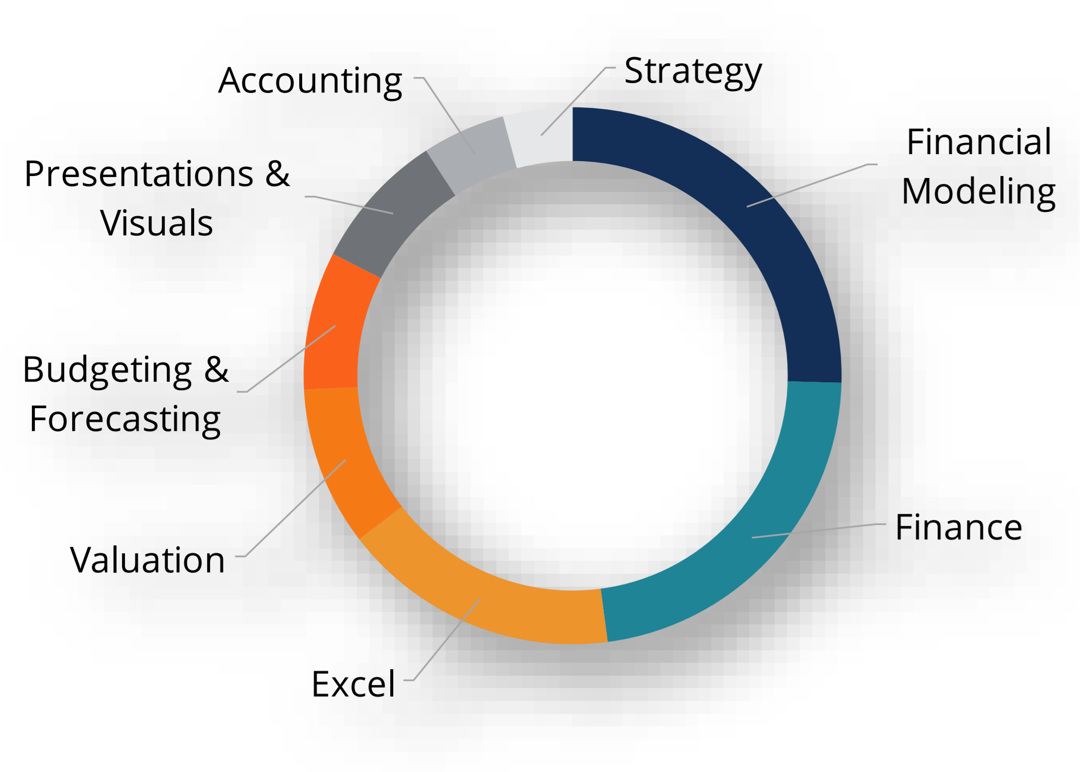
A well rounded financial analyst possesses all of the above skills!
CFI is the global institution behind the financial modeling and valuation analyst FMVA® Designation. CFI is on a mission to enable anyone to be a great financial analyst and have a great career path. In order to help you advance your career, CFI has compiled many resources to assist you along the path.
In order to become a great financial analyst, here are some more questions and answers for you to discover:


